How much time does this cast have left on stage?

by Scott Sereday

Last Tuesday, Andrew wrote about the winter of the Duncan Dynasty in San Antonio. His article was pessimistic about how much the current core could contribute to an additional championship, saying “the league passed San Antonio by.’Â Of course, this pessimism is not entirely unfounded.

The Spurs haven’t won the vaunted NBA title since 2007. Duncan is 34. Ginobili is 33 and Parker is 28 and coming off an injury-plagued season. Andrew is probably right to suggest tempered expectations, but do these lowered expectations mean that the Spurs should rebuild? I suspect few will suggest rebuilding until there are very strong signs of decline from at least 2 of the Big 3. After all, the arthritic Celtics came tantalizing close to their second championship in 3 years this past June.

If the current group of Spurs isn’t at the end of the line, how much longer do they have?

Measurement tools

In order to estimate how much each player can be expected to contribute to a team’s future, I utilized statistical performances over the last two years and age as of December 31, 2010. I measured each player’s expected contribution using Mean Expected Championships Added (MECA). MECA is the estimate of the expected championships above average a player would be expected to win if he was removed from his team and randomly placed on any team in the NBA.

Total MECA doesn’t equal total championships won for two reasons. First, a player can collect a ring simply by being on the right team without any measurable positive contributions to the team. For this reason, poor players tend to have more championships than MECA. Secondly, using the Lakers as an example, one might say that since the Finals were so hotly contested, the Lakers without Kobe Bryant would have had a 30% chance of the winning the 2010 title. In this case, we can say he created 0.7 championships (this doesn’t mean his MECA is 0.7 because MECA adjusts for all potential teams and only accounts for the regular season, but the same logic applies).

However, we could also say that the Lakers without Pau Gasol (but with Kobe) may have only had a 30% chance of repeating. Before estimating the other players’ championships added, we can see that adding Kobe’s and Pau’s championships created already exceeds the number of actual championships won. The more appropriate way to measure championships added is to always determine each player’s impact on point differential, adding them together (with slight adjustments) and then converting this new adjustment to wins and then championships. We might find that the Lakers with neither Kobe or Pau would have a 5% chance at a title.

Data for Statistical Plus Minus

In order to be able to project future career expectations, I excluded all players who played this past season so that each observation had “completed career results.” I used data beginning with the 1979/80 season. I estimated each players performance over the last two years using Advanced Statistical Plus Minus (ASPM). This is an estimate of a player’s value using box score and play-by-play statistics (see articles on Offensive and Defensive ASPM for further explanation). I weighed 2010 two times as heavily as 2009 (also weighing by minutes for each respective season).

In order to account for players like Garrett Temple and Alonzo Gee, who only played a handful of minutes, I established a credibility factor for the weighted minutes. For players whose 2010 minutes * 2 + 2009 minutes exceed 10,000, I used the pure estimate described above. Those whose minutes came in less than 10,000, I applied a factor accounting for the data’s credibility to the the initial estimate and added the remaining percentage multiplied by -3, which is approximately the average player’s ASPM. This factor is (total weighted minutes/10,000)^0.5.

I’ll use Mr. Duncan to illustrate how this is applied. Tim Duncan played 2,525 minutes with a 6.3 ASPM in 2009 and 2,435 with a 5.1 ASPM in 2010. His resulting initial estimate is (6.3*2,525 + 5.1*2,435*2)/(2,525 + 2,435*2) = 5.5. His total weighted minutes is equal to 2,525 + 2,435*2 = 7,395, which means the initial estimate must be adjusted by (7,395/10,000)^0.5 = 0.86. Finally, 0.86*(-3) is added to the total. Duncan’s final 2 year weighted ASPM is 5.5*0.86 - 3*0.14 = 4.3. For prediction purpose, this weighted value predicts 2011 ASPM with higher accuracy than only using 2010 ASPM.

Graphing Statistical Plus Minus and age against MECA

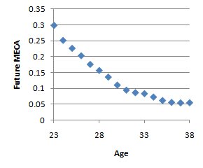
Now that I have a reasonable estimation of a player’s expected value, I can utilize this 2-year weighted ASPM, supplemented with player age, to predict future MECA. Taking the average future MECA for each player of all respective ages and excluding all ages with fewer than 15 observations, I can produce the following graph displaying future MECA as age increases:

Similarly, the following graph shows how future MECA changes with increases to ASPM:

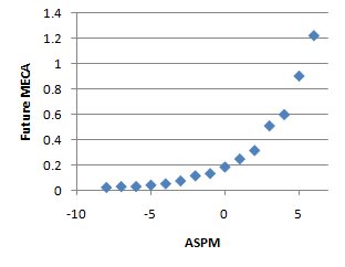
The most obvious feature apparent from observing these graphs is the curved progression of each. MECA decreases at a slower rate as players age and increases faster with improvements to ASPM. Unlike my last post, in which I performed simple linear regression analysis (notice the straight trend line of the graph), a log transformation should be applied to the dependent variable (future expected MECA is dependent on ASPM and Age) in order to appropriately fit the data. This log transformation simply means that I chose the best regression model fitting the natural log of MECA. The Graphs look much more linear after this adjustment.

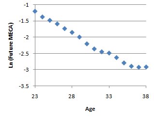
Keep in mind the end values have fewer observations and are more innately variable.

Summary of Results

Fitting both independent variables (ASPM and Age) to the log transformation of Future MECA, the regression model of 2.95-0.179*Age+0.449*ASPM-0.017*Max(ASPM,0)^1.5 can be used to predict ln(Future MECA). Converting this to something more meaningful, Tim Duncan’s estimate of future MECA can be estimated by e^(3.36-0.179*34+0.497*4.3-0.084*4.3^1.5) = 2.718^(-1.338) = 0.262.

The results of the other Spurs can be observed in the table below (I have also entered an estimate of future seasons, assuming all of these players play this upcoming season):

PLAYER	POS	Age	Yrs	Career MECA	2010 ASPM	2009 ASPM	Adj 2yr ASPM	Alt ASPM	Future Span	Future MECA	Alt Future MECA
Manu Ginobili	SG	33	8	1.192	7.5	8.6	5.4	5.0	6.9	0.400	0.367
George Hill	PG	24	2	0.069	-1.7	0.8	-0.5	0.5	9.0	0.306	0.488
Tim Duncan	C	34	13	2.379	6.3	5.1	4.3	5.0	5.9	0.262	0.307
DeJuan Blair	PF	21	1	0.019		-1.2	-2.0	-1.0	9.9	0.248	0.408
Matt Bonner	PF	30	6	0.191	3.6	1.5	0.6	0.5	6.3	0.174	0.167
Tony Parker	PG	28	9	0.376	3.8	-2.8	-0.7	3.5	6.8	0.135	0.630
Alonzo Gee	SG	23	1	0.008		-1.0	-2.6	-1.0	8.6	0.129	0.285
Garrett Temple	SG	24	1	0.012		-1.6	-2.6	-1.0	8.0	0.108	0.239
Richard Jefferson	SF	30	9	0.412	0.1	-1.2	-1.0	0.0	5.6	0.082	0.134
Antonio McDyess	PF	36	14	0.345	2.1	-5.2	-2.7	-1.0	1.7	0.012	0.028

Before I discuss the results, I want to point out the importance of remembering that all statistical analysis should be sandwiched between non-statistical reasoning. Usually, the process starts with a question and the experiment is designed to answer that question. In the least, the experiment should provide clarification for an observed issue in question.

Next is the statistical analysis, which often takes the longest. Once results can be determined, the outputs are observed and the design is adjusted in an attempt to make the results more meaningful, obvious or interesting. Finally, the most important part is bringing the numbers back to reality. With new information, one needs to understand the potential driving forces contributing to these results. Sometimes, aspects that aren’t accounted for should be added to the conclusion. The interpretation can be different from person-to-person. None of them are completely right, but some of them are useful and closer to the truth than others.

Conclusions

Getting back to the above table, we see that Ginobili projects the highest, followed by George Hill, Duncan, DeJuan Blair, Matt Bonner and Tony Parker. However, we should keep in mind that this is a basic approximation of expectations. The most glaring problem with these numbers is that they do not focus on the fact that Parker’s number last year were likely hampered by injury. If we assume that he will be unaffected by past injuries, it’s reasonable to project his as the brightest future of anyone on this list.

As you see, Ginobili typically turns out pretty well in most statistical analysis. Of course, this statistical analysis doesn’t adequately account for man-to-man defense, especially on the perimeter. Ginobili’s defensive reputation doesn’t nearly match his sterling defensive numbers and if you consider him to be a subpar man defender, his defensive value would likely be overrated (I’m not completely convinced either way at this point). Additionally, Manu’s minutes tend to be lower than expected based on his value per play and if this trend continues, his value will likely be lower than his projections. DeJuan Blair projects well due to his young age and solid contributions last year, but this projection doesn’t factor in concerns about his knees.

Statistical similarity tests are another common method used for projections. This works well in some cases, but in my opinion, often focuses too much on results when the causes of these results might be more indicative of how a player ages. For example, looking at Tim Duncan I suspected he might age well since he relies on height and skills rather than athleticism. However, the list of statistically similar players tends to include players like Patrick Ewing, Alonzo Mourning, Artis Gilmore, Larry Nance, Kevin McHale and David Robinson. Unlike Duncan, Mourning, Nance and Robinson relied significantly on athleticism and Gilmore was several inches taller. Most of these players also seemed to have better natural outside shooting ability than Duncan.

I suspect that visual observations of player similarities should still play a significant role in player projections given the current state of available data. Robert Parish seems to best represent Duncan’s makeup of athleticism, shooting ability and length. Parish’s teammate, McHale also seems have many of the same skills and much of the same makeup as Duncan. However, at Duncan’s current age of 34, McHale began to suffer from injuries that likely brought his career to a premature halt. There is reason for optimism with Duncan’s longevity, but injuries can always be an issue, especially for older players. In my opinion, Parker seems to relate best to a combination of Isiah Thomas, without the same passing ability, and Andrew Toney (whose career also suffered from injuries).

Ginobili seems difficult to peg but might be most comparable to Clyde Drexler, Sidney Moncrief (another great player whose effectiveness was severely limited due to injuries) and Mitch Richmond. It’s interesting to note that with all these comparable players, several have been hampered by injuries late in their career. Perhaps a reduction in minutes for the big 3 will help preserve them for several more years.